Ray theory is the infinite-frequency approximation of time-harmonic wave theory. The partial differential equation governing ray theory is the eikonal equation, which is obtained by taking the high-frequency limit of the Helmholtz equation \begin{align}\label{eq:helmholtz} \nabla^2 p + k^2 p =0\,, \end{align} where \(k = \omega/c\) is the wavenumber, \(\omega\) is the angular frequency, and \(c\) is the sound speed.
Inserting \(p(\vec{x}) = P(\vec{x},\omega)e^{i\omega \tau(\vec{x})}\) into Eq. \eqref{eq:helmholtz}, writing \(\nabla^2 = \vec{\nabla}\cdot \vec{\nabla}\), and evaluating the gradient yields \begin{align} \divergence [e^{i\omega \tau(\vec{x})} \gradient P(\vec{x},\omega) + i\omega P(\vec{x},\omega) e^{i\omega \tau(\vec{x})} \gradient\tau(\vec{x})] + k^2 P(\vec{x},\omega)e^{i\omega \tau(\vec{x})} = 0\,. \label{eq:helmholtz:1} \end{align} Taking the divergence of the quantity in square brackets in Eq. \eqref{eq:helmholtz:1} yields \begin{align} &i\omega e^{i\omega \tau(\vec{x})} \gradient \tau(\vec{x}) \cdot \gradient P(\vec{x},\omega) + e^{i\omega \tau(\vec{x})}\Laplacian P(\vec{x},\omega) \notag\\ &\quad + i\omega \gradient [P(\vec{x},\omega) e^{i\omega \tau(\vec{x})}] \cdot \gradient\tau(\vec{x}) + i\omega P(\vec{x},\omega)e^{i\omega \tau(\vec{x})}\Laplacian\tau(\vec{x}) + k^2 P(\vec{x},\omega)e^{i\omega \tau(\vec{x})} = 0\,.\label{eq:helmholtz:2} \end{align} where the vector calculus identity \begin{align}\label{eq:id:1} \divergence [f(\vec{x})\gradient {g}(\vec{x})] = \gradient f(\vec{x}) \cdot \gradient {g}(\vec{x}) + f(\vec{x}) \Laplacian g(\vec{x}) \end{align} has been used. Evaluating the gradient of the quantity in square brackets in the second line of Eq. \eqref{eq:helmholtz:2} yields \begin{align} &i\omega \gradient \tau(\vec{x}) \cdot \gradient P(\vec{x},\omega) + \Laplacian P(\vec{x},\omega) \notag\\ &\quad + i\omega\gradient P(\vec{x},\omega)\cdot \gradient\tau(\vec{x}) - \omega^2 P(\vec{x},\omega) \gradient \tau(\vec{x}) \cdot \gradient\tau(\vec{x}) + i\omega P(\vec{x},\omega)\Laplacian\tau(\vec{x}) + k^2 P(\vec{x},\omega) = 0\,. \end{align} Grouping common terms, writing \(k^2 = \omega^2/c^2\), and suppressing the functional dependencies on position and frequency yields [1, Eq. (8.5.1)] \begin{align}\label{1} \Laplacian P + i\omega (2 \gradient P\cdot \gradient \tau + P\Laplacian\tau) - \omega^2 P\left[(\gradient \tau)^2 - \tfrac{1}{c^2}\right] &= 0\,. \end{align} Substituting the asymptotic expansion \(P(\vec{x},\omega) = P_0(\vec{x}) + \omega^{-1} P_1(\vec{x}) + \omega^{-2} P_2(\vec{x}) + \dots\) into Eq. \eqref{1} yields \begin{align} \Laplacian &[P_0(\vec{x}) + \omega^{-1} P_1(\vec{x}) + \omega^{-2} P_2(\vec{x}) + \dots] \notag \\ &+ i 2 \gradient [\omega P_0(\vec{x}) + P_1(\vec{x}) + \omega^{-1} P_2(\vec{x}) + \dots]\cdot \gradient \tau + i[\omega P_0(\vec{x}) + P_1(\vec{x}) + \omega^{-1} P_2(\vec{x})+ \dots]\Laplacian\tau \notag \\ &- [\omega^2 P_0(\vec{x}) + \omega P_1(\vec{x}) + P_2(\vec{x}) + \dots]\left[(\gradient \tau)^2 - \tfrac{1}{c^2}\right] = 0\,.\label{eq:1:sub} \end{align} If \(\omega\) is very large, the terms of order \(\omega^{-1}\), \(\omega^{-2}\), and higher are very small. Also, \(\omega P_0 \gg P_1\) and \(\omega^2 P_0 \gg \omega P_1 \gg P_2 \) for large \(\omega\). Thus Eq. \eqref{eq:1:sub} approximately equals \begin{align} %\Laplacian P_0(\vec{x}) + i 2 \gradient \omega P_0(\vec{x})\cdot \gradient \tau + i\omega P_0(\vec{x})\Laplacian\tau \notag - \omega^2 P_0(\vec{x})\left[(\gradient \tau)^2 - \tfrac{1}{c^2}\right] &= 0\,.\label{eq:1:sub:lim} \\ \Laplacian P_0 + i\omega (2 \gradient P_0\cdot \gradient \tau + P_0\Laplacian\tau) - \omega^2 P_0\left[(\gradient \tau)^2 - \tfrac{1}{c^2}\right] &= 0\,. \label{eq:1:sub:lim} \end{align} In the \(\omega \to \infty\) limit, Eq. \eqref{eq:1:sub:lim} separates into three independent equations: \begin{alignat}{2} \nabla^2 P_0(\vec{x}) &=0\,, \qquad && O(\omega^0) \,, \label{eq:omega:0}\\ 2 \gradient P_0 \cdot \gradient \tau + P_0 \Laplacian \tau &=0\,, \qquad && O(\omega^1) \,, \label{eq:omega:1}\\ P_0\left[(\gradient \tau)^2 - \tfrac{1}{c^2}\right] &=0\,, \qquad && O(\omega^2)\,. \label{eq:omega:2} \end{alignat} The emergence of Eq. \eqref{eq:omega:0} is somewhat surprising, since the the Laplace equation is associated with the low-frequency approximation \((k \to 0)\) of Eq. \eqref{eq:helmholtz} [2, p. 492]. Although Eq. \eqref{eq:omega:0} is superfluous to the present discussion, the mathematical connection between zero- and infinite-frequency wave phenomena is interesting [and I do not think Pierce discusses Eq. \eqref{eq:omega:0} in this context].
The \(\omega^1\) and \(\omega^2\) equations, in contrast, describe wave propagation at infinite frequencies. The \(\omega^2\) equation [1, Eq. (8.5.3a)] \begin{align} \boxed{(\gradient \tau)^2 = \frac{1}{c^2}}\label{eq:eikonal} \end{align} is known as the eikonal equation, about which Pierce writes,
Once any wavefront surface is specified and a value of \(\tau\) is associated with it, the value of \(\tau(\vec{x})\) for any position \(\vec{x}\) can be determined by finding that ray connecting the originally specified wavefront with the point \(\vec{x}\). If the ray passes through point \(\vec{x}_0\) on the originally specified wavefront, and if \(\tau(\vec{x}_0) = \tau_0\), \(\tau(\vec{x})\) is \(\tau_0\) plus the travel time at speed \(c\) along the ray from \(\vec{x}_0\) to \(\vec{x}\).
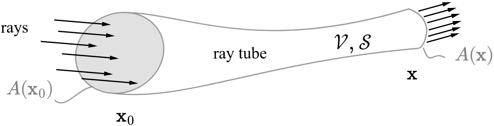
Suppose that rays in the immediate vicinity of position \(\vec{x}_0\) pass through a cross-sectional area \(A(\vec{x}_0)\) whose unit normal coincides with the direction of the rays. The same rays near another position \(\vec{x}\) pass through a cross-sectional area \(A(\vec{x})\). The areas \(A(\vec{x}_0)\) and \(A(\vec{x})\) define the ends of a ray tube whose sides are everywhere parallel to the direction of the rays. Let the volume defined by the ray tube be denoted by \(\mathcal{V}\), while the surface be denoted by \(\mathcal{S}\). Integration of Eq. \eqref{3b*} over \(\mathcal{V}\) results in \(\int_{\mathcal{V}} \divergence (P^2 \gradient \tau)\, dV = 0\), and application of the divergence theorem yields \begin{align}\label{eq:surf} \oint_{\mathcal{S}} (P^2 \gradient \tau) \cdot \vec{n}\, dS = 0 \,, \end{align} where \(\vec{n}\) is the outward unit normal vector to the surface. Since the walls of the ray tube are parallel to the direction of the rays, the only contributions to the surface integral in Eq. \eqref{eq:surf} are the values of the integrand at the ends, resulting in \begin{align}\label{eq:ray:alg} (P^2 \gradient \tau \cdot \vec{n})\big\rvert_{\vec{x}} \, A(\vec{x}) - (P^2 \gradient \tau \cdot \vec{n})\big\rvert_{\vec{x}_0} \, A(\vec{x}_0) = 0 \,. \end{align} Pierce notes that \(\gradient \tau\cdot \vec{n} = 1/c\), which is now assumed to be the same at points \(\vec{x}_0\) and \(\vec{x}\). The assumption that \(c\) is the same at points \(\vec{x}_0\) and \(\vec{x}\) implies that the medium is homogeneous, and that the rays travel in straight lines [The ray tube depicted above (adapted from Pierce's Fig. 8.17) therefore has no curvature for the following result to hold]. Thus Eq. \eqref{eq:ray:alg} becomes \(P^2(\vec{x}) A(\vec{x}) = P^2(\vec{x}_0) A(\vec{x}_0)\), which, upon taking the square root of both sides and solving for \(x_0\), gives \begin{align}\label{eq:amp} \boxed{P(\vec{x}) = P(\vec{x}_0) \sqrt{\frac{A(\vec{x}_0)}{A(\vec{x})}}\,.} \end{align} Equation \eqref{eq:amp} describes how the amplitude varies along a ray tube.