Diffraction

Chapters 13-14: Diffraction

This section is almost entirely based on my class notes from Dr. Hamilton's Acoustics II course. The derivations are challenging, so hints/outlines have been provided. It is more important to understand the underlying concepts.

How does the quantity \(R = |\vec{r}- \vec{r}_0|\) relate a sound source to the listener? [answer]

If the source is located at \(\vec{r}_0\) and the listener is located at \(\vec{r}\), \(R = |\vec{r}- \vec{r}_0|\) is the distance between source and listener. Its shorthand when appearing in the argument of a Green's function is \(\vec{r}|\vec{r}_0\).
☸ Prove that the free space Green's function \(g = e^{-jkR}/4\pi R\) solves the inhomogeneous Helmholtz equation \((\nabla^2 + k^2)f = -\delta(\vec{r} - \vec{r}_0)\), where \(R = |\vec{r}- \vec{r}_0|\). Hint: Integrate the differential equation over the volume of a sphere of radius \(\epsilon\) and use the divergence theorem to convert the volume integral into a surface integral. Evaluate the surface integral and then take the limit as \(\epsilon \to 0\). Also note that \(\int_0^\epsilon e^{-jkR} R dR \to 0 \text{ as } \epsilon \to 0\). [answer]

Inserting the Green's function into the Helmholtz equation and integrating over space gives \begin{align*} \int \nabla^2 g dV + k^2 \int g \, dV &= -1 \end{align*} The divergence theorem is applied to the first integral: \begin{align*} \int \nabla^2 g dV &= \int \gradient\cdot(\gradient g) dV\\ &= \oint \gradient g\, dS. \end{align*} Since at radius \(R = \epsilon\) the differential area is \(dS = \epsilon^2 d\theta\,d\psi\), the equation above becomes \begin{align*} \int \nabla^2 g dV &= \int_0^{2\pi} \int_{0}^\pi \left(\frac{dg}{dR}\right)_{R=\epsilon} \epsilon^2\, d\theta \,d\psi \\ &= 4\pi \epsilon^2 \left[\frac{d}{dR}\bigg(\frac{e^{-jkR}}{4\pi R}\bigg)\right]_{R=\epsilon}\\ &= 4\pi \epsilon^2 \left[\bigg(-\frac{1}{4\pi R^2} - \frac{jk}{4\pi R}\bigg)e^{-jkR}\right]_{R=\epsilon}\\ &= -(1 + jk\epsilon)\, e^{-jk\epsilon} \end{align*} Now the limit of the above result is taken: \begin{align*} -\lim_{\epsilon\to 0} (1 + jk\epsilon)e^{-jk\epsilon} &= -\lim_{\epsilon\to 0} (1 + jk\epsilon)(1 - jk\epsilon -k^2\epsilon^2/2! \dots)\\ &=-1\,. \end{align*} Meanwhile, the second integral is \begin{align*} \int \frac{e^{-jkR}}{4\pi R} dV &= \int_0^\epsilon \frac{e^{-jkR}}{4\pi R} 4\pi R^2 dR\\ &= \int_0^\epsilon e^{-jkR} R dR \to 0 \text{ as } \epsilon \to 0\,. \end{align*} Thus one obtains the true statement, \(-1 = -1\). The free space Green's function thus satisfies the inhomogeneous Helmholtz equation.
What is reciprocity in acoustics? [answer]

Reciprocity is the invariance under the exchange of sound source and listener. That is to say, the listener perceives the same sound when exchanging locations with the source of that sound.
To determine the condition that makes a medium reciprocal, suppose there are point sources at positions \(\vec{r}_1\) and \(\vec{r}_2\). The free space Green's functions \(G(\vec{r}|\vec{r}_1)\) and \(G(\vec{r}|\vec{r}_2)\) satisfy their respective inhomogeneous Helmholtz equations. Combination of the Helmholtz equations, integration over volume, and application of the divergence theorem leads to \begin{align}\label{vanishitofffthat}\tag{13} \int_{\mathcal{S}} \bigg[G(\vec{r}|\vec{r}_2) \frac{\partial G(\vec{r}|\vec{r}_1)}{\partial n} - G(\vec{r}|\vec{r}_1) \frac{\partial G(\vec{r}|\vec{r}_2)}{\partial n}\bigg] dS &= G(\vec{r}_2|\vec{r}_1) - G(\vec{r}_1|\vec{r}_2)\,. \end{align} Why does the right-hand side of equation (\ref{vanishitofffthat}) equal \(0\)? What are the three conditions on the boundary of surface \(\mathcal{S}\) in which the left-hand side vanishes, thereby satisfying the equality and giving the conditions for a reciprocal medium? [answer]

The right-hand side of equation (\ref{vanishitofffthat}) equals \(0\) because the free space Green's function is even in the quantity \(\vec{r}_2 - \vec{r}_1\).

The left-hand side vanishes for \begin{align} G &= 0 \label{Greenboundary1}\tag{i}\\ \frac{\partial G}{\partial n} &= 0 \label{Greenboundary2}\tag{ii}\\ \frac{\partial G/\partial n}{G} &= \text{ constant}\,. \label{Greenboundary3}\tag{iii} \end{align} Boundary condition (\ref{Greenboundary1}) corresponds to a pressure release surface; (\ref{Greenboundary2}) corresponds to a rigid surface; and (\ref{Greenboundary3}) corresponds to the Sommerfeld radiation condition or a locally reacting surface.
☸ Starting with the Helmholtz equation for a point-inhomogeneity,\(\nabla^2 G + k^2 G = -\delta(\vec{r} - \vec{r}_0)\), and for a function-inhomogeneity, \(\nabla^2 p + k^2 p = -f(\vec{r})\), derive the Helmholtz-Kirchhoff integral, \begin{align}\label{HKint}\tag{14} p(\vec{r}) = \int_{\mathcal{V}} f(\vec{r}_0) G(\vec{r}|\vec{r}_0)dV_0 + \oint_\mathcal{S} \bigg[G(\vec{r}|\vec{r}_0) \frac{\partial p(\vec{r}_0)}{\partial n_0} - p(\vec{r}_0)\frac{\partial G(\vec{r}|\vec{r}_0)}{\partial n_0} \bigg]dS_0 \end{align} Outline: Relate the two PDEs by multiplying the point-inhomogeneity PDE by \(p\) and the function-inhomogeneity PDE by \(G\). Subtract, interchange \(\vec{r}\) and \(\vec{r}_0\), integrate over volume, and apply the divergence theorem. Why does the surface integral vanish in free space? [answer]

Start with \begin{align} \nabla^2 p(\vec{r}) + k^2 p(\vec{r}) &= -f(\vec{r}) \tag{i}\label{1equation}\\ \nabla^2 G(\vec{r}|\vec{r}_0) + k^2 G(\vec{r}|\vec{r}_0) &= -\delta(\vec{r} - \vec{r}_0)\,. \tag{ii}\label{2equation} \end{align} Multiply equation (\ref{1equation}) by \(G\) and equation (\ref{2equation}) by \(p\), and subtract the two equations. The \(k^2\) terms cancel, giving \begin{align*} G(\vec{r}|\vec{r}_0)\nabla^2 p(\vec{r}) - p(\vec{r}) \nabla^2 G(\vec{r}|\vec{r}_0) &= -f(\vec{r}) G(\vec{r}|\vec{r}_0) + \delta(\vec{r} - \vec{r}_0) p(\vec{r}) \end{align*} Next, interchange \(\vec{r}\) and \(\vec{r}_0\) and integrate over volume \(V_0\). Note that \(G\) cares not about this exchange, nor does the delta function. \begin{align*} \int_{\mathcal{V}} [G(\vec{r}|\vec{r}_0)\nabla^2_0 p(\vec{r}_0) - p(\vec{r}_0) \nabla^2_0 G(\vec{r}|\vec{r}_0)] dV_0 &= \int_{\mathcal{V}} [\delta(\vec{r} - \vec{r}_0) p(\vec{r}_0)-f(\vec{r}_0) G(\vec{r}|\vec{r}_0) ] dV_0\\ &= p(\vec{r}) - \int_{\mathcal{V}}f(\vec{r}_0) G(\vec{r}|\vec{r}_0) ] dV_0\,. \end{align*} Finally, using the divergence theorem on the left-hand side above reduces the Laplacian operators to derivatives on the normal. Solving for \(p(\vec{r})\) results in the Helmholtz-Kirchhoff integral: \[p(\vec{r}) = \int_{\mathcal{V}} f(\vec{r}_0) G(\vec{r}|\vec{r}_0)dV_0 + \int_\mathcal{S} \bigg[G(\vec{r}|\vec{r}_0) \frac{\partial p(\vec{r}_0)}{\partial n_0} - p(\vec{r}_0)\frac{\partial G(\vec{r}|\vec{r}_0)}{\partial n_0} \bigg]dS\]

If the medium is reciprocal, the surface integral vanishes in free space because \(p = 0\) at \(r= \infty\), giving the pressure due to a distribution of sources in free space: \[p(\vec{r}) = \int_{\mathcal{V}} f(\vec{r}_0) G(\vec{r}|\vec{r}_0)dV_0 \]
☸ Use equation (\ref{HKint}) to derive the Rayleigh integral of the first kind, \begin{align}\label{Rayleigh integral}\tag{15} p(\vec{r}) &= \frac{j\omega \rho_0}{2\pi}\oint_\mathcal{S} \frac{e^{-jkR}}{R} u^{(z)}(\vec{r}_0) dS_0 \end{align} which gives the pressure field due to a velocity source. Let \(\vec{e}_{n0}\) be the unit outward normal, and align the surface source in the plane \(z=0\), as shown below. Outline: Let the first integral in equation (\ref{HKint}) be zero, i.e., assume no sources distributed in the volume. With the remaining surface integral, write \(\partial p(\vec{r}_0)/\partial n_0 = -\partial p(\vec{r}_0)/\partial z_0\) in terms of particle velocity using the momentum equation. With the second term, choose \(G\) such that \(\partial G/\partial n_0 = 0\) on the surface. The correct choice (show this) is \(G(\vec{r}|\vec{r}_0) = g_+(\vec{r}|\vec{r}_0) + g_-(\vec{r}|\vec{r}_0)\), where \(g_\pm = e^{-jkR_\pm}/4\pi R_\pm\), where \(R_\pm = \sqrt{(x-x_0)^2 + (y-y_0)^2 + (z\mp z_0)^2}\). [answer]

Let the first integral in equation (\ref{HKint}) be zero, i.e., assume no sources are distributed in the volume: \begin{align} p(\vec{r}) &= \oint_\mathcal{S} \bigg[G(\vec{r}|\vec{r}_0) \frac{\partial p(\vec{r}_0)}{\partial n_0} - p(\vec{r}_0)\frac{\partial G(\vec{r}|\vec{r}_0)}{\partial n_0} \bigg]dS_0\notag\\ &= \oint_\mathcal{S} \bigg[-G(\vec{r}|\vec{r}_0) \frac{\partial p(\vec{r}_0)}{\partial z_0} + p(\vec{r}_0)\frac{\partial G(\vec{r}|\vec{r}_0)}{\partial z_0} \bigg]\bigg\rvert_{z_0=0}dS_0\label{HKint1}\tag{i} \end{align} Since an equation that maps particle velocity to pressure is desired, write \(\partial p(\vec{r}_0)/\partial n_0\) in terms of particle velocity using the momentum equation. \begin{align*} \frac{\partial p(\vec{r}_0)}{\partial n_0} = -\frac{\partial p(\vec{r}_0)}{\partial z_0} = j\omega \rho_0 u^{(n)}(\vec{r}_0) \end{align*} Next, choosing \(G(\vec{r}|\vec{r}_0) = g_+(\vec{r}|\vec{r}_0) + g_-(\vec{r}|\vec{r}_0)\), where \(g_\pm = e^{-jkR_\pm}/4\pi R_\pm\), where \[R_\pm = \sqrt{(x-x_0)^2 + (y-y_0)^2 + (z\mp z_0)^2},\] note that \begin{align*} \frac{\partial G}{\partial z_0}\bigg\rvert_{z_0=0}&= \frac{\partial g_+}{\partial z_0}\bigg\rvert_{z_0=0} + \frac{\partial g_-}{\partial z_0}\bigg\rvert_{z_0=0}\\ &=\frac{\partial }{\partial z_0}\frac{e^{-jkR_+}}{4\pi R_+}\bigg\rvert_{z_0=0} + \frac{\partial}{\partial z_0}\frac{e^{-jkR_-}}{4\pi R_-}\bigg\rvert_{z_0=0}\\ &=\bigg[\frac{jke^{-jkR_+}(z-z_0)}{4\pi R_+^2} + \frac{(z-z_0)}{4\pi R_+^3}e^{-jkR_+} -\frac{jke^{-jkR_-}(z+z_0)}{4\pi R_-^2} - \frac{(z+z_0)}{4\pi R_-^3}e^{-jkR_-} \bigg]_{z=0} \end{align*} Note that for \(z_0=0\), \(R_+ = R_-\equiv R\), and the above equation becomes \begin{align} \frac{\partial G}{\partial z_0}\bigg\rvert_{z_0=0}&=\frac{jke^{-jkR}(z-z_0)}{4\pi R^2} + \frac{(z-z_0)}{4\pi R^3}e^{-jkR} -\frac{jke^{-jkR}(z+z_0)}{4\pi R^2} - \frac{(z+z_0)}{4\pi R^3}e^{-jkR}\notag\\ &=0\tag*{woohoo!} \end{align} Also, \(g_+ = g_- \equiv g\) at \(z_0=0\), so \(G = 2g = e^{-jkR/4\pi R}\). So equation (\ref{HKint1}) becomes \begin{align*} p(\vec{r}) &= \oint_\mathcal{S} \bigg(\frac{2e^{-jkR}}{4\pi R}\bigg) \big[j\omega \rho_0 u^{(r)}\big] dS_0 \end{align*} Rearranging gives the famous Rayleigh integral of the first kind of acoustics (and the second kind of optics): \begin{align*} p(\vec{r}) &= \frac{j\omega \rho_0}{2\pi}\oint_\mathcal{S} \frac{e^{-jkR}}{R} u^{(r)}(\vec{r}_0) dS_0 \end{align*} In Cartesian coordinates, \begin{align*} p(x,y,z) &= \frac{j\omega \rho_0}{2\pi}\iint_{-\infty}^\infty \frac{e^{-jkR}}{R} \, u^{(r)}(x_0,y_0,0) \,dx_0\, dy_0\,. \end{align*} where \(R = \sqrt{(x-x_0)^2 + (y-y_0)^2 +z^2}\). Note that the contour integral symbol \(\oint\) denoting "integral over a closed surface" is abandoned because there is no sound incident on the surface infinitely far away. (This relates to the Sommerfeld radiation condition).
Use the Rayleigh integral for a velocity source, Eq. (\ref{Rayleigh integral}) to calculate the on-axis (\(x=y=0\)) field due to a uniform circular piston of radius \(a\). [answer]

Setting \(x = y =0\) in Cartesian coordinates corresponds to setting \(\sigma=0\) in cylindrical coordinates in the Rayleigh integral, Eq. (\ref{Rayleigh integral}), and thus \(R = \sqrt{\sigma_0^2 + z^2}\). Also, since the field is axisymmetric, \(u^{(z)}(\vec{r}_0) = u^{(z)}(\sigma_0)\). Eq. (\ref{Rayleigh integral}) therefore becomes \begin{align*} p(0,z) &= \frac{j\omega \rho_0}{2\pi}\int_{0}^{2\pi}\!\! \int_{0}^{\infty} \frac{e^{-jkR}}{R} u^{(z)}(\sigma_0) \sigma_0 d\sigma_0 d\theta \\ &= \frac{jk\rho_0c_0u_0}{2\pi}\int_{0}^{2\pi}\!\! \int_{0}^{a} \frac{e^{-jk\sqrt{\sigma_0^2 + z^2}}}{\sqrt{\sigma_0^2 + z^2}} \sigma_0 d\sigma_0 d\theta\,. \end{align*} The radial integral contains no \(\theta\) dependence. Thus \begin{align*} p(0,z) &= jk\rho_0c_0u_0\int_{0}^{a} \frac{e^{-jk\sqrt{\sigma_0^2 + z^2}}}{\sqrt{\sigma_0^2 + z^2}} \sigma_0 d\sigma_0 \,. \end{align*} Letting \(s = \sqrt{\sigma_0^2 + z^2}\) and thus \(ds = \sigma_0 d\sigma_0/\sqrt{\sigma_0^2 + z^2}\), the radial integral is evaluated: \begin{align*} p(0,z) &= jk\rho_0c_0u_0\int_{z}^{\sqrt{a^2 + z^2}} e^{-jks} ds \\ &= -\rho_0c_0 u_0 \exp(-jks)\bigg\rvert_{z}^{\sqrt{a^2+z^2}}\\ &= \rho_0c_0 u_0 [\exp(-jkz) - \exp(-jk\sqrt{a^2+z^2})]\,. \end{align*} The above can be factorized as \begin{align*} p(0,z) &= \rho_0c_0 u_0 \exp\bigg[\frac{jk}{2}(-z - \sqrt{a^2+z^2})\bigg] \bigg\lbrace\exp\bigg[\frac{jk}{2}(-z + \sqrt{a^2+z^2})\bigg] - \exp\bigg[\frac{jk}{2}(z - \sqrt{a^2+z^2})\bigg]\bigg\rbrace\,. \end{align*} Recalling that \((e^{jx}-e^{-jx})/2j = \sin x\), the above becomes \begin{align*} p(0,z) &= 2j\rho_0c_0 u_0 \exp[-jk(z + \sqrt{a^2+z^2})/2] \sin[k(\sqrt{a^2+z^2} - z)/2] \,. \end{align*} The magnitude of this expression is \begin{align*} |p(0,z)| &= 2\rho_0c_0 u_0 \big|\sin[k(\sqrt{a^2+z^2}-z)/2]\big| \,. \end{align*}
☸ Derive the Rayleigh integral of the second kind, \begin{align}\label{Rayleigh integral 2}\tag{16} p(\vec{r}) &= \frac{jkz}{2\pi} \oint p(\vec{r}_0) \bigg(1 + \frac{1}{jkR} \bigg) \frac{e^{-jkR}}{R^2} dS_0\,, \end{align} which gives the pressure field due to a pressure source. Start with equation (\ref{HKint}), and follow the derivation for the first Rayleigh integral, only now choosing \(G(\vec{r}|\vec{r}_0) = g_+(\vec{r}|\vec{r}_0) - g_-(\vec{r}|\vec{r}_0)\). What is this integral called in optics? [answer]

As in the derivation of the first Rayleigh integral, let the first integral in equation (\ref{HKint}) be zero, i.e., assume no sources are distributed in the volume. Since an equation that maps pressure to pressure is desired, it is desired for \(\partial G(\vec{r}|\vec{r}_0)/\partial n_0\) to vanish on the boundary. Choosing \(G(\vec{r}|\vec{r}_0) = g_+(\vec{r}|\vec{r}_0) - g_-(\vec{r}|\vec{r}_0)\) does the trick, because at the \(z=0\), \(R_+ = R_- \equiv R\), and thus \(g_+ = g_- \equiv g\), so \begin{align*} G(\vec{r}|\vec{r}_0)\bigg\rvert_{z_0=0} = g(\vec{r}|\vec{r}_0) - g(\vec{r}|\vec{r}_0)= 0\,. \end{align*} Thus the Helmholtz-Kirchhoff integral becomes \begin{align} p(\vec{r}) &= \oint_\mathcal{S} p(\vec{r}_0)\frac{\partial G(\vec{r}|\vec{r}_0)}{\partial z_0}\bigg\rvert_{z_0=0} dS_0\notag\\ &= \oint p(x_0,y_0,0) \bigg[\frac{\partial }{\partial z_0}\frac{e^{-jkR_+}}{4\pi R_+} - \frac{\partial}{\partial z_0}\frac{e^{-jkR_-}}{4\pi R_-}\bigg] \bigg\rvert_{z_0=0} dx_0dy_0\tag{ii}\label{suberherslkdf} \end{align} Note that the term in the square brackets is evaluated separately to be \begin{align*} \bigg[\dots\bigg]&=\bigg[\frac{jke^{-jkR_+}(z-z_0)}{4\pi R_+^2} + \frac{(z-z_0)}{4\pi R_+^3}e^{-jkR_+} +\frac{jke^{-jkR_-}(z+z_0)}{4\pi R_-^2} + \frac{(z+z_0)}{4\pi R_-^3}e^{-jkR_-} \bigg]_{z_0=0}\\ &= \frac{jke^{-jkR}z}{4\pi R^2} + \frac{z}{4\pi R^3}e^{-jkR} +\frac{jke^{-jkR}z}{4\pi R^2} + \frac{z}{4\pi R^3}e^{-jkR}\\ &= \frac{jke^{-jkR}z}{2\pi R^2} + \frac{z}{2\pi R^3}e^{-jkR}\\ &= \frac{jkz}{2\pi} \bigg(1 + \frac{1}{jkR} \bigg) \frac{e^{-jkR}}{R^2} \end{align*} Thus equation (\ref{suberherslkdf}) becomes \begin{align*} p(\vec{r}) &= \frac{jkz}{2\pi} \oint p(\vec{r}_0) \bigg(1 + \frac{1}{jkR} \bigg) \frac{e^{-jkR}}{R^2} dS_0\,, \end{align*} or in Cartesian coordinates, \begin{align*} p(x,y,z) &= \frac{jkz}{2\pi} \iint_{-\infty}^\infty p(x_0,y_0,0) \bigg(1 + \frac{1}{jkR} \bigg) \frac{e^{-jkR}}{R^2} dx_0dy_0 \end{align*} where \(R=\sqrt{(x-x_0)^2 + (y-y_0)^2 +z^2}\). Again, the contour integral symbol \(\oint\) denoting "integral over a closed surface" is abandoned because there is no sound incident on the surface infinitely far away.

This integral is called the Rayleigh integral of the first kind in optics because (need to confirm) usually in optics the source condition is given in terms of the field variable. That is to say, \(E(x_0,y_0,0)\) is used to compute \(E(x,y,z)\), while or \(H(x_0,y_0,0)\) is used to compute \(H(x,y,z)\).
☸ Obtain the Fraunhofer approximation of the Rayleigh integral of the first kind (\ref{Rayleigh integral}): \begin{align}\label{Fraunhofer}\tag{17} p(\vec{r}) &= \frac{j\omega \rho_0}{2\pi}\frac{e^{-jkr}}{r} \iint_{-\infty}^\infty e^{jk_xx_0 + jk_yy_0} u_0(x_0,y_0) dx_0 dy_0 \end{align} Outline: Expand the squares in the displacement \(R = \sqrt{(x-x_0)^2 + (y-y_0)^2 +z^2},\) identify \(r^2 = x^2+ y^2+z^2\), and take the first-order binomial expansion of \(R\). Multiply by \(k\) to make the quantity dimensionless, and throw out quadratic terms (terms proportional to \(x_0^2,y_0^2\)). Finally, interpret \(k_x \equiv kx/r\) and \(k_y \equiv ky/r\). Do you recognize the resulting 2D integral? At what \(r\) does the Fraunhofer approximation hold? [answer]

Begin by expanding \(R\): \begin{align*} R &= \sqrt{(x-x_0)^2 + (y-y_0)^2 +z^2}\\ &= \big[x^2 + y^2 + z^2 -2xx_0 - 2yy_0 + x_0^2 + y_0^2\big]^{1/2}\\ &= \big[r^2 -2xx_0 - 2yy_0 + x_0^2 + y_0^2\big]^{1/2}\\ &= r \bigg[1 -2 \frac{xx_0 + yy_0}{r^2} + \frac{x_0^2 + y_0^2}{r^2} \bigg]^{1/2}\\ \end{align*} Now perform the binomial expansion to first order: \begin{align*} R&= r \bigg[1 - \frac{xx_0 + yy_0}{r^2} + \frac{x_0^2 + y_0^2}{2r^2}\bigg]\\ &= r - \frac{xx_0 + yy_0}{r} + \frac{x_0^2 + y_0^2}{2r} \,. \end{align*} Next, multiply by \(k\) to make the quantity dimensionless (and because this is the combination that appears in the Rayleigh integral), and toss the term that is quadratic: \begin{align*} kR &= kr - kx_0\frac{x}{r} - ky_0\frac{y}{r}\\ &=kr - k_x x_0 - k_y y_0\,. \end{align*} where the interpretation \(k_x \equiv kx/r\) and \(k_y \equiv ky/r\) has been made. Approximate the amplitude in equation (\ref{Rayleigh integral}) to zeroth order and the phase to linear order: \begin{align*} p(\vec{r}) &= \frac{j\omega \rho_0}{2\pi}\frac{e^{-jkr}}{r} \iint_{-\infty}^\infty e^{jk_xx_0 + jk_yy_0} u_0(x_0,y_0) dx_0 dy_0 \end{align*} (Note that the notation changes here from denoting the velocity source condition from \(u^{(r)}\) to \(u_0\)). The integral above is simply the 2D spatial Fourier transform of the source condition. This is often denoted \(\hat{u}(k_x,k_y)\). The directivity is defined as \[D(\theta,\psi) = \frac{\hat{u}_0(k_x,k_y)}{\hat{u}_0(0,0)}.\]

The Fraunhofer approximation holds for \(r \gtrsim 3R_0\), where \(R_0= ka^2/2\), the Rayleigh distance.
What is the \(ka \ll 1\) limit of the Fraunhofer approximation? [answer]

In this limit the exponential in equation (\ref{Fraunhofer}) \(\to 1\). Thus the 2D spatial Fourier transform simply becomes the surface integral over the velocity source condition, which is \(Q_0\), the volume velocity. Thus the \(ka \ll 1\) limit of the Fraunhofer approximation is an acoustic monopole: \[p(\vec{r}) = \frac{j\omega \rho_0 Q_0}{2\pi} \frac{e^{-jkr}}{r}\,.\]
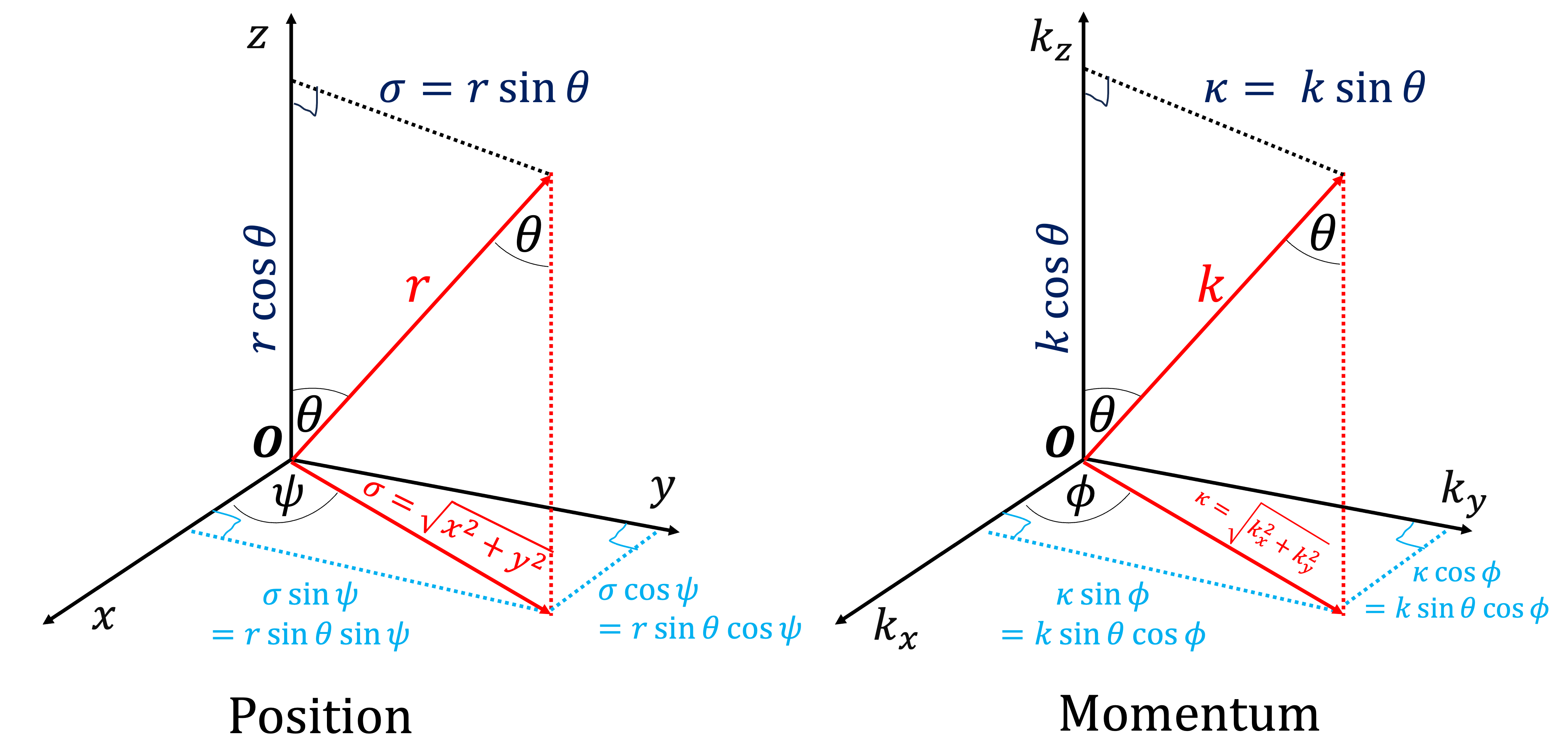
Convert the Fraunhofer approximation, equation (\ref{Fraunhofer}), which is given in terms of rectangular coordinates in the source plane, to polar coordinates in the source plane using the change-of-variables in which \(\kappa = k\sin\theta\), and \begin{alignat*}{2} x&= \sigma \cos \psi \qquad y&&= \sigma \sin \psi \\ k_x&= \kappa\cos \phi \qquad k_y&&= \kappa\sin \phi\,. \end{alignat*} Then simplify the result to the case of an axisymmetric beam (no dependence on \(\psi\)). [answer]

The argument of the exponential in the integrand of equation (\ref{Fraunhofer}) becomes \begin{align*} k_xx_0 + k_yy_0 &= \kappa\cos \phi\,\,\,\sigma_0 \cos \psi_0 \,\,\, + \,\,\, \kappa\sin \phi\,\,\, \sigma_0 \sin \psi_0 \\ &= \kappa\sigma_0 (\cos \phi\,\,\cos \psi_0 \, + \, \sin \phi\,\, \sin \psi_0)\\ &= \kappa\sigma_0 \cos(\phi -\psi_0) \end{align*} Also, \(dx_0\,dy_0 = \sigma_0\, d\sigma_0\, d\psi_0 \). Thus equation (\ref{Fraunhofer}) becomes \begin{align*} p(\vec{r}) &= \frac{j\omega \rho_0}{2\pi}\frac{e^{-jkr}}{r} \int_{0}^{2\pi}\int_{0}^{\infty} e^{j\kappa\sigma_0 \cos(\phi -\psi_0)} u_0(\sigma_0,\psi_0) \, \sigma_0\, d\sigma_0 d\psi_0\\ &= \frac{j\omega \rho_0}{2\pi}\frac{e^{-jkr}}{r} \int_{0}^{2\pi} e^{j\kappa\sigma_0 \cos(\phi -\psi_0)} d\psi_0 \int_{0}^{\infty} u_0(\sigma_0)\, \sigma_0\, d\sigma_0 \end{align*} The first line above is the farthest the Fraunhofer approximation can be taken if the source condition has an angular dependence (e.g., a vortex beam). In the second line, it has been assumed that \(u_0 = u_0(\sigma_0)\). In that case, identify \(2\pi\, J_0(\kappa \sigma_0) = \int_{0}^{2\pi} e^{j\kappa\sigma_0 \cos(\phi -\psi_0)} d\psi_0\), i.e., an integral representation of the Bessel function. Thus \begin{align*} p(\vec{r}) &= \frac{j\omega \rho_0}{2\pi}\frac{e^{-jkr}}{r} \bigg[2\pi \int_{0}^{\infty} J_0(\kappa \sigma_0) u_0(\sigma_0) \,\sigma_0 \, d\sigma_0 \bigg] \end{align*} The integral above is the Hankel transform, denoted \(\hat{u}_{0,H}(\kappa)\), and the quantity in brackets \([\dots]\) is \(2\pi\, \hat{u}_{0,H}(\kappa)\), which is simply the Fourier transform. Also, note that \(J_0(0) = 1\). Thus the volume velocity is given by \(\hat{u}_{0,H}(0) = Q_0 = 2\pi \int_{0}^{\infty} u_0(\sigma_0) \,\sigma_0 \, d\sigma_0\). Multiplying and dividing by the volume velocity gives \begin{align*} p(\vec{r}) &= \frac{j\omega \rho_0 Q_0}{2\pi}\frac{e^{-jkr}}{r} \frac{2\pi \int_{0}^{\infty} J_0(\kappa \sigma_0) u_0(\sigma_0) \,\sigma_0 \, d\sigma_0}{2\pi \int_{0}^{\infty} u_0(\sigma_0) \,\sigma_0 \, d\sigma_0}\\ &=\frac{j\omega \rho_0 Q_0}{2\pi}\frac{e^{-jkr}}{r} \frac{2\pi \int_{0}^{\infty} J_0(\kappa \sigma_0) u_0(\sigma_0) \,\sigma_0 \, d\sigma_0}{\hat{u}_{0,H}(0)} \end{align*} The pressure field is thus written in terms of the directivity \(D(\theta)\): \begin{align*} p(\vec{r}) &= \frac{j\omega \rho_0 Q_0}{2\pi}\frac{e^{-jkr}}{r}D(\theta) \\ D(\theta) &= \frac{\hat{u}_{0,H}(\kappa)}{\hat{u}_{0,H}(0)} \end{align*}
Find the far-field pressure field and directivity due to a thin ring of pressure at \(z=0\) centered about the \(z\) axis, given by the condition \begin{align*} u_0(\sigma) = u_0 w \delta(\sigma-a) \end{align*} where \(\sigma\) is the radial coordinate in the source plane. [answer]

Recall from the previous question that the pressure field is given by \begin{align*} p(\vec{r}) &= \frac{j\omega \rho_0 Q_0}{2\pi}\frac{e^{-jkr}}{r}D(\theta) \\ D(\theta) &= \frac{\hat{u}_{0,H}(\kappa)}{\hat{u}_{0,H}(0)} \end{align*} where the Hankel transform is defined as \begin{align*} \hat{u}_{0,H}(\kappa) = \int_{0}^{\infty} J_0(\kappa \sigma_0) u_0(\sigma_0) \,\sigma_0 \, d\sigma_0\,. \end{align*} Letting \(u_0(\sigma) = u_0 w \delta(\sigma-a)\), the Hankel transform is calculated using the sifting property of the delta function: \begin{align*} \hat{u}_{0,H}(\kappa) &= u_0 w \, \int_{0}^{\infty} J_0(\kappa \sigma_0) \delta(\sigma-a) \,\sigma_0 \, d\sigma_0\\ &= u_0 w a \, J_0(\kappa a) \end{align*} Thus \(\hat{u}_{0,H}(0) = u_0 w a\). So the far-field directivity is given by \[D(\theta) = J_0(\kappa a) = J_0 (ka\sin\theta)\,,\] and the pressure in the far field is given by \begin{align*} p(\vec{r}) &= \frac{j\omega \rho_0 Q_0}{2\pi}\frac{e^{-jkr}}{r} J_0 (ka\sin\theta)\,. \end{align*}
Find the far-field pressure field and directivity due to a uniform circular piston at \(z=0\) centered about the \(z\) axis, given by the condition \begin{align*} u_0(\sigma) = \begin{cases} u_0,\quad \sigma \in [0,a] \\ 0,\quad \sigma > a \end{cases}\,, \end{align*} where \(\sigma\) is defined as before. [answer]

Recall from the previous two questions that the pressure field is given by \begin{align*} p(\vec{r}) &= \frac{j\omega \rho_0 Q_0}{2\pi}\frac{e^{-jkr}}{r}D(\theta) \\ D(\theta) &= \frac{\hat{u}_{0,H}(\kappa)}{\hat{u}_{0,H}(0)} \end{align*} where the Hankel transform is \(\hat{u}_{0,H}(\kappa) = \int_{0}^{\infty} J_0(\kappa \sigma_0) u_0(\sigma_0) \,\sigma_0 \, d\sigma_0\). Letting \(u_0(\sigma) = u_0\) for \(\sigma \in [0,a]\) and \(0\) for \(\sigma > a\), the Hankel transform is calculated: \begin{align*} \hat{u}_{0,H}(\kappa) &= u_0 \, \int_{0}^{a} J_0(\kappa \sigma_0) \,\sigma_0 \, d\sigma_0\\ &= u_0 a^2 \frac{J_1(\kappa a)}{\kappa a}\,. \end{align*} Since \(\lim_{x\to 0} J_1(x)/x = 1/2\), \(\hat{u}_{0,H}(0) = u_0 a^2/2\). So the far-field directivity is given by \[D(\theta) = \frac{2J_1(\kappa a)}{\kappa a} = \frac{2J_1(ka\sin\theta)}{ka\sin\theta} \,,\] and the pressure in the far field is \begin{align*} p(\vec{r}) &= j\rho_0 c_0 u_0 \frac{ka^2}{2}\frac{e^{j(\omega t - kr)}}{r} \frac{2J_1(ka\sin\theta)}{ka\sin\theta}\,. \end{align*}
☸ Obtain the Fresnel (paraxial) approximation of equation (\ref{Rayleigh integral}). The result is \begin{align}\label{Fresnel}\tag{18} p(x,y,z) &= \frac{j\omega \rho_0}{2\pi}\frac{e^{-jkz}}{z}\iint_{-\infty}^\infty \, u_0(x_0,y_0) e^{-jk [(x-x_0)^2 + (y-y_0)^2]/2z}\,dx_0\, dy_0\,. \end{align} Outline: Expand \(R\) in powers of \(1/z\) (whereas in the Fraunhofer approximation, \(R\) was expanded in powers of \(1/r\)). What are the limits on this approximation? [answer]

Start with the first Rayleigh integral, given by equation (\ref{Rayleigh integral}), where \[R = \sqrt{(x-x_0)^2 + (y-y_0)^2 +z^2}\,.\] As in the Fraunhofer approximation, \(R\) is the quantity that is approximated. However, this time it is expanded in powers of \(1/z\): \begin{align*} R &= z\bigg[{1 + \frac{(x-x_0)^2}{z^2} + \frac{(y-y_0)^2}{z^2}}\bigg]^{1/2} \end{align*} The quadratic terms are considered to be small, and the binomial expansion is applied: \begin{align*} R &= z\bigg[{1 + \frac{(x-x_0)^2}{2z^2} + \frac{(y-y_0)^2}{2z^2}}\bigg]\\ &=z + \frac{(x-x_0)^2}{2z} + \frac{(y-y_0)^2}{2z} \end{align*} The denominator of the integrand of equation (\ref{Rayleigh integral}) is approximated to zeroth order as \(z\). Meanwhile, the quantity \(kR\) that appears in the exponent becomes \begin{align*} kR &= kz + \frac{k}{2z}\big[(x-x_0)^2 + (y-y_0)^2\big] \end{align*} Note that the next higher order term would be \(\mathcal{O}(z^{-3}) \sim ka^4/8z^3\) which is declared to be \(\ll \pi\), i.e., the \(\mathcal{O}(z^{-3})\) does not contribute significantly to the phase of \(e^{-jkR}\), giving the criterion for the paraxial approximation to be \((z/a)^3 \gtrsim ka/8\pi\), or simply \(z/a \gtrsim (ka)^{1/3}\), which corresponds to a region defined by a \(\pm 20^\circ\) angle about the \(z\) axis (the paraxial region). Thus the first Rayleigh integral becomes \begin{align*} p(x,y,z) &= \frac{j\omega \rho_0}{2\pi}\frac{e^{-jkz}}{z}\iint_{-\infty}^\infty \, u_0(x_0,y_0) e^{-jk [(x-x_0)^2 + (y-y_0)^2]/2z}\,dx_0\, dy_0\,. \end{align*} where \(u^{(r)}(x_0,y_0,0)\) has been notated \(u_0(x_0,y_0)\) for simplicity. This is known as the "Fresnel diffraction integral." However, it should not be called the "Fresnel integral," which refers to an integral involved in the diffraction of waves about semi-infinite screens or double-rectangular apertures.
Does the paraxial approximation depend on \(ka\)? Does the paraxial approximation contain evanescent waves? [answer]

While the paraxial approximation is entirely independent of \(ka\), an implicit assumption underlying the paraxial approximation is that \(ka \gg 1\). This condition keeps the wavefronts quasi-planar. The "plane wave part" of the Fresnel diffraction integral is the factor \(e^{-ikz}\) in front of the integral.

The paraxial approximation does not contain evanescent waves. This can be seen by noting that the quantity \begin{align*} kR &= kz + \frac{k}{2z}\big[(x-x_0)^2 + (y-y_0)^2\big] \end{align*} is purely real-valued and becomes purely imaginary when multiplied by \(-j\) in the exponential \(e^{-jkR}\). Thus there are only exponentials of imaginary arguments, which correspond to propagating waves. (In contrast, recall that evanescent waves correspond to exponentials of real arguments).
Obtain the axisymmetric form of equation (\ref{Fresnel}), using the rectangular-to-polar mapping \begin{alignat*}{2} x&= \sigma \cos \psi \quad x_0 &&= \sigma_0 \cos\psi_0\\ y&= \sigma \sin \psi \quad y_0 &&= \sigma_0 \sin\psi_0 \end{alignat*} and thus \(dx_0 dy_0 = \sigma_0 d\sigma_0 d\psi_0\). Denote \(\omega \) as \(kc_0\). [answer]

Begin with the rectangular form of the Fresnel diffraction integral, equation (\ref{Fresnel}), only with \(\omega\) denoted as \(kc_0\): \begin{align*} p(x,y,z) &= \frac{jk \rho_0 c_0}{2\pi}\frac{e^{-jkz}}{z}\iint_{-\infty}^\infty \, u_0(x_0,y_0) e^{-jk [(x-x_0)^2 + (y-y_0)^2]/2z}\,dx_0\, dy_0, \end{align*} and note that \begin{align*} (x-x_0)^2 + (y-y_0)^2 &= \sigma^2 \cos^2 \psi + \sigma_0^2 \cos^2\psi_0 - 2\sigma\sigma_0 \cos \psi \cos \psi_0 \\ &\quad + \sigma^2 \sin^2 \psi + \sigma_0^2 \sin^2\psi_0 - 2\sigma\sigma_0 \sin\psi \sin\psi_0\\ &= \sigma^2 + \sigma_0^2 - 2\sigma \sigma_0 (\cos \psi \cos\psi_0 + \sin\psi \sin\psi_0)\\ &= \sigma^2 + \sigma_0^2 - 2\sigma \sigma_0 \cos(\psi -\psi_0) \end{align*} Thus the Fresnel diffraction integral becomes \begin{align*} p(\sigma,\psi,z) &= \frac{jk \rho_0 c_0}{2\pi}\frac{e^{-jkz}}{z}\int_{0}^{2\pi} \int_{0}^\infty \, u_0(\sigma_0,\psi_0) e^{-jk [\sigma^2 + \sigma_0^2 - 2\sigma \sigma_0 \cos(\psi -\psi_0)]/2z}\,\sigma_0\,d\sigma_0\, d\psi_0 \,. \end{align*} This is as far as one can go if \(u_0\) depends on the polar angle \(\psi_0\). If \(u_0\) does not depend on this angle, the above becomes \begin{align*} p(\sigma, \psi, z) &= \frac{jk \rho_0 c_0}{2\pi}\frac{e^{-jkz}}{z}e^{-jk\sigma^2/2z} \int_{0}^\infty u_0(\sigma_0) e^{-jk\sigma_0^2/2z}\sigma_0\,d\sigma_0\, \int_{0}^{2\pi} e^{j(k\sigma \sigma_0/z) \cos(\psi -\psi_0)}\, d\psi_0 \end{align*} The polar integral is an integral representation of the Bessel function. It equals \(2\pi J_0 (k\sigma \sigma_0/z)\). Thus \begin{align}\label{Fresnelaxi}\tag{i} p(\sigma, \psi, z) &= e^{-jkz} \bigg[\frac{jk \rho_0 c_0}{z}e^{-jk\sigma^2/2z} \int_{0}^\infty u_0(\sigma_0) J_0 (k\sigma \sigma_0/z) e^{-jk\sigma_0^2/2z}\sigma_0\,d\sigma_0\bigg]\,. \end{align} Note that equation (\ref{Fresnelaxi}) is of the form \(p = q e^{-jkz}\), where \(q\) is the quantity in \([\dots]\) above. This \(q\) is the quantity that is slowly varying in \(z\), and \(e^{-jkz}\) is simply the plane wave propagator.
How does one include spherical focusing in the Fresnel approximation? Let the focal length be \(d\). Then a spherical wavefront is proportional to \(e^{jk\sqrt{x^2 + y^2 + (z-d)^2}}/\sqrt{x^2 + y^2 + (z-d)^2}\). Let the aperture \(a/d\) be small, where \(a\) is the source radius. [answer]

Start with the spherical wave condition at \(z=0\), the source: \(e^{jk\sqrt{x^2 + y^2 + d^2}}/\sqrt{x^2 + y^2 + d^2}\). Then phase is \begin{align*} jk[x^2 + y^2 + d^2]^{1/2} &= jkd\bigg[ 1 + \frac{x^2 + y^2}{d^2} \bigg]^{1/2}\\ &\simeq jkd + jk\frac{x^2 + y^2}{2d}\,, \end{align*} and the magnitude is simply \begin{align*} [x^2 + y^2 + d^2]^{-1/2} &= \frac{1}{d}[1 + (x^2 + y^2)/d^2]^{-1/2}\simeq \frac{1}{d} \end{align*} Thus focused wave is proportional to \(\frac{e^{jkd}}{d} e^{jk(x_0^2+y_0^2)/2d}\) in the Fresnel approximation, and accounting for focusing simply amounts to a multiplication of the Fresnel diffraction integral by \(e^{jk(x_0^2+y_0^2)/2d}\). In polar coordinates, the focusing factor is \(e^{jk\sigma_0^2/2d}.\) That is, the Fresnel diffraction integral becomes \begin{align*} p(\sigma,\psi,z) &= \frac{jk \rho_0 c_0}{2\pi}\frac{e^{-jkz}}{z}\int_{0}^{2\pi} \int_{0}^\infty \, u_0(\sigma_0,\psi_0) e^{jk\sigma_0^2/2d} e^{-jk [\sigma^2 + \sigma_0^2 - 2\sigma \sigma_0 \cos(\psi -\psi_0)]/2z}\,\sigma_0\,d\sigma_0\, d\psi_0\,, \,. \end{align*} or, for an axisymmetric beam, \begin{align*} p(\sigma, \psi, z) &= e^{-jkz} \bigg[\frac{jk \rho_0 c_0}{z}e^{-jk\sigma^2/2z} \int_{0}^\infty u_0(\sigma_0) J_0 (k\sigma \sigma_0/z) e^{jk\sigma_0^2/2d} e^{-jk\sigma_0^2/2z}\sigma_0\,d\sigma_0\bigg]\,. \end{align*}
In the paraxial approximation, the field in the focal plane of a focused source is given by the ________ transform of the source condition in cartesian coordinates and the ________ transform in polar coordinates. Why is this? [answer]

(2D spatial) Fourier; Hankel. This is because at \(z = d\), the factor \(e^{-jk\sigma_0^2/2z}\) equals \(e^{-jk\sigma_0^2/2d}\), which cancels out with the focusing factor \(e^{jk\sigma_0^2/2z}\), leaving \(\int_0^\infty u_0(\sigma_0) J_0(k\sigma \sigma_0/d)\sigma_0 d\sigma_0\) [the Hankel transform of \(u_0(\sigma_0)\)] as the integral in the paraxial approximation. For source conditions that are not axisymmetric, the integral is the 2D spatial Fourier transform of the source condition, though it takes more algebra to show this.
Derive the paraxial wave equation, \[-j2k\frac{\partial q}{\partial z} + \nabla^2_\perp q= 0\,,\] where \(\nabla^2_\perp\) is the transverse Laplacian, \(\partial/\partial x^2 + \partial/\partial y^2\) in Cartesian coordinates. Start with the Helmholtz equation, \(\nabla^2 p + k^2 p = 0\), and let \(p(x,y,z) = q(x,y,z)e^{-jkz}\). Note that \(\partial^2 q/\partial z^2 \ll 1\). [answer]

Take the derivatives of \(p\), and let subscripts indicate partial differentiation with respect to the subscripted variable. By inspection, \begin{align*} \frac{\partial^2 p}{\partial x^2} = q_{xx}e^{-jkz}\quad \text{and}\quad \frac{\partial^2 p}{\partial y^2} = q_{yy}e^{-jkz}\,. \end{align*} Meanwhile, \begin{align*} \frac{\partial p}{\partial z} &= q_z e^{-jkz} -jk q e^{-jkz} = (q_z -jk q)e^{-jkz}\\ \frac{\partial^2 p}{\partial z^2} &= (q_{zz} -jk q_z)e^{-jkz} - jk (q_z -jk q) e^{-jkz}\\ &=(q_{zz} - j2k q_z - k^2 q) e^{-jkz} \end{align*} The Helmholtz equation in Cartesian coordinates, \(p_{xx} + p_{yy} + p_{zz} + k^2 p = 0\), becomes \begin{align*} q_{xx} e^{-jkz} + q_{yy}e^{-jkz} + (q_{zz} - j2k q_z - k^2 q) e^{-jkz} + k^2 q e^{-jkz} &= 0\\ q_{xx} + q_{yy} + (q_{zz} - j2k q_z - k^2 q) + k^2 q &= 0\\ q_{xx} + q_{yy} + q_{zz} - j2k q_z &= 0\,. \end{align*} Noting that \(q_{zz} \) is small (Dr. Hamilton showed this rigorously in class), and denoting \(\partial/\partial x^2 + \partial/\partial y^2 \equiv \nabla^2_\perp\), results in \[-j2k\frac{\partial q}{\partial z} + \nabla^2_\perp q= 0\,.\]
State Babinet's principle. [answer]

Babinet's principle says that "complementary diffracting objects have complementary diffraction patterns" (Blackstock, page 484). For example, the complementary diffracting object of a finite disk of radius \(a\) in free space is a circular aperture of radius \(a\). Babitnet's principle says that the sum of the radiation patterns individually caused by the finite disk and the aperture must be the same as the radiation pattern of the beam in free space.
The \(i(kx-\omega t)\) convention is adopted for this problem. Use the 2D Fourier transform pair \(\hat{f}(k_x,k_y) = \iint_{-\infty}^\infty f(x,y) e^{-i(k_xx+ k_yy)\,dxdy}\) and \({f}(x,y) = (2\pi)^{-2}\iint_{-\infty}^\infty \hat{f}(k_x,k_y) e^{i(k_xx+ k_yy)\,dk_xdk_y}\) to solve the Helmholtz equation in terms of the source condition \(p(x,y,z=0)\). Hint: note that the Fourier transform of the \(n^\mathrm{th}\) derivative of \(f\) with respect to \(x\) is \((ik_x)^n \hat{f}(k_x,k_y)\), and that the \(n^\mathrm{th}\) derivative of \(f\) with respect to \(y\) is \((ik_y)^n \hat{f}(k_x,k_y)\). Use these relations to reduce the Helmholtz equation to an second-order ordinary differential equation in \(z\). How does the solution change for a velocity source? [answer]

See here for the solution.

↑ Return to physical acoustics ← Return to previous topic → Advance to next topic