Ultrasonics

Elasticity

This section is based on the first chapter of Introduction to Elastic Wave Propagation by Bedford and Drumheller.

What is the difference between \(\vec{X}\) and \(\vec{x}\)? Quantities written in terms of \(\vec{X}\) belong in the ____________ description while quantities written in terms of \(\vec{x}\) belong in the ____________ description. Which description is more conventionally used in acoustics, and which is more conventionally used in elasticity? [answer]

\(\vec{X}\) is the position vector of an object in the reference state, while \(\vec{x}\) is the position vector of an object in the current state. Quantities written in terms of \(\vec{X}\) belong in the Lagrangian (material) description while quantities written in terms of \(\vec{x}\) belong in the Eulerian (spatial) description. The Lagrangian description is more commonly used in elasticity, because deformations of an object are studied with respect to the initial state, where the Eulerian description is more common in acoustics because microphones measure Eulerian quantities.
Use Cartesian index notation, i.e., \(\vec{X} \mapsto X_k\), \(\vec{x} \mapsto x_k\), \(k = 1,2,3\). Define the motion and inverse motion. [answer]

The motion is defined as \[x_k = \hat{x}_k(X_m, t)\,,\] where the "hat" indicates that a function depends on the variables \(X_k\) and \(t\). The inverse motion is defined as \[X_k = X_k(x_m, t)\,.\]
The displacement is defined as \(\vec{u} = \vec{x}- \vec{X}\). The velocity is the time derivative of the displacement, and the acceleration is the time derivative of the velocity. Evaluate the displacement, velocity, and acceleration in the Lagrangian and Eulerian desciptions. [answer]

See here for the definitions.
Noting that \[dx_k = \frac{\partial \hat{x}_k}{\partial X_m}\, dX_m\,,\] and defining \begin{align*} dS^2&= dX_k \, dX_k\\ ds^2&= dx_k \, dx_k = \frac{\partial \hat{x}_k}{\partial X_m}\, dX_m\, \frac{\partial \hat{x}_k}{\partial X_n}\, dX_n\,, \end{align*} show that \[ds^2-dS^2 = 2E_{mn} dX_m dX_n,\] where \[E_{mn} = \frac{1}{2}\bigg(\frac{\partial \hat{u}_m}{\partial X_n} + \frac{\partial \hat{u}_n}{\partial X_m} + \frac{\partial \hat{u}_k}{\partial X_m} \frac{\partial \hat{u}_k}{\partial X_n}\bigg)\,. \] What is \(E_{mn}\) called? [answer]

Using the provided definitions, \begin{align*} ds^2-dS^2 = \frac{\partial \hat{x}_k}{\partial X_m}\, dX_m\, \frac{\partial \hat{x}_k}{\partial X_n}\, dX_n - dX_k \, dX_k \end{align*} The \(dX_mdX_n\) term can be factored out by using a Kronecker delta \(\delta_{mn}\) in the second term: \begin{align*} ds^2-dS^2 = \bigg(\frac{\partial \hat{x}_k}{\partial X_m}\, \, \frac{\partial \hat{x}_k}{\partial X_n}\, - \delta_{mn}\bigg) dX_m\,dX_n\,. \end{align*} Now the definition of the Lagrangian displacement, \(\hat{u}_k = \hat{x}_k - X_k\), or \(\hat{x}_k = \hat{u}_k + X_k\), is invoked: \begin{align*} ds^2-dS^2 &= \bigg[\frac{\partial}{\partial X_m}(\hat{u}_k + X_k)\, \, \frac{\partial}{\partial X_n}(\hat{u}_k + X_k)\, - \delta_{mn}\bigg] dX_m\,dX_n\\ &= \bigg[\bigg(\frac{\partial \hat{u}_k}{\partial X_m} + \frac{\partial X_k}{\partial X_m}\bigg)\, \bigg(\frac{\partial \hat{u}_k}{\partial X_n} + \frac{\partial X_k}{\partial X_n}\bigg)\, - \delta_{mn}\bigg] dX_m\,dX_n\\ &= \bigg[\bigg(\frac{\partial \hat{u}_k}{\partial X_m} + \delta_{km}\bigg)\, \bigg(\frac{\partial \hat{u}_k}{\partial X_n} + \delta_{kn}\bigg)\, - \delta_{mn}\bigg] dX_m\,dX_n\\ &= \bigg[\frac{\partial \hat{u}_k}{\partial X_m}\frac{\partial \hat{u}_k}{\partial X_n} + \frac{\partial \hat{u}_k}{\partial X_n}\delta_{km} + \frac{\partial \hat{u}_k}{\partial X_m}\delta_{kn}\bigg] dX_m\,dX_n\\ &= \bigg[\frac{\partial \hat{u}_m}{\partial X_n} + \frac{\partial \hat{u}_n}{\partial X_m} + \frac{\partial \hat{u}_k}{\partial X_m}\frac{\partial \hat{u}_k}{\partial X_n} \bigg] dX_m\,dX_n\\ \end{align*} Defining the Lagrangian strain tensor \[E_{mn} = \frac{1}{2}\bigg(\frac{\partial \hat{u}_m}{\partial X_n} + \frac{\partial \hat{u}_n}{\partial X_m} + \frac{\partial \hat{u}_k}{\partial X_m} \frac{\partial \hat{u}_k}{\partial X_n}\bigg)\,, \] the final equation above reads \[ds^2-dS^2 = 2E_{mn} dX_m dX_n.\] In linear elasticity, the Lagrangian strain tensor becomes \[E_{mn} = \frac{1}{2}\bigg(\frac{\partial {u}_m}{\partial x_n} + \frac{\partial {u}_n}{\partial x_m}\bigg)\,,\] or in index notation, \[E_{mn} = \frac{1}{2}({u}_{m,n} + {u}_{n,m})\,. \]
To what does the stress-strain relation \(T_{km} = c_{kmij} E_{ij}\) reduce for isotropic linear elastic materials? [answer]

\[T_{km} = \lambda \delta_{km} E_{jj} + 2\mu E_{km}.\] \(\lambda\) is the dilation constant, and \(\mu\) is the shear modulus.

Derivation of elastic wave equation

See section 1.6 of Bedford and Drumheller for a more thorough development of Newton's second law and its linearization.

The linearized differential form of Newton's second law in the absence of body forces reads \[\rho a_m = \frac{\partial T_{mk}}{\partial x_k}\,.\] In linear elasticity the left-hand side can be written as \(\rho a_m = \rho_0 \partial^2 u_m/\partial t^2\), while the stress tensor for a linear isotropic material, upon substitution of the linear strain tensor, becomes \[T_{mk} = \lambda \delta_{mk} \frac{\partial u_j}{\partial x_j} + \mu \bigg(\frac{\partial u_m}{\partial x_k} + \frac{\partial u_k}{\partial x_m} \bigg)\,.\] Obtain \[\rho_0 \frac{\partial^2 \vec{u}}{\partial t^2} = (\lambda +\mu) \vec{\nabla}(\vec{\nabla}\cdot \vec{u}) + \mu \nabla^2 \vec{u} \] by combining Newton's second law and the linear strain tensor. [answer]

Inserting \[T_{mk} = \lambda \delta_{mk} \frac{\partial u_j}{\partial x_j} + \mu \bigg(\frac{\partial u_m}{\partial x_k} + \frac{\partial u_k}{\partial x_m} \bigg)\,.\] into the right-hand side of \[\rho a_m = \frac{\partial T_{mk}}{\partial x_k}\,\] gives \[\rho_0 \frac{\partial^2 u_m}{\partial t^2} = (\lambda +\mu) \frac{\partial^2 u_k}{\partial x_k \partial x_m} + \mu \frac{\partial^2 u_m}{\partial x_k \partial x_k}\,,\] which in vector form gives the desired result.
The vector Laplacian identity \(\nabla^2 \vec{A} = \vec{\nabla}(\vec{\nabla} \cdot \vec{A}) - \vec{\nabla}\times (\vec{\nabla}\times \vec{A})\) can be used to write the result of question (1) above as \[\rho_0 \frac{\partial^2 \vec{u}}{\partial t^2} = (\lambda +2 \mu) \vec{\nabla}(\vec{\nabla}\cdot \vec{u}) - \mu \vec{\nabla}\times (\vec{\nabla} \times \vec{u}) \] Apply the Helmholtz decomposition \(\vec{u} = \vec{\nabla} \phi + \vec{\nabla}\times \vec{\psi}\) to the above to obtain two wave equations, one corresponding to compressional waves, and the other corresponding to shear waves. Which one travels faster? [answer]

See here for the decomposition. The compressional wave travels faster, as can be seen from the expression for the sound speed.

Relflection and transmission

What are the boundary conditions at the boundary of two media for normally incident compressional waves? Use knowledge from Acoustics I to immediately write the stress- reflection and transmission coefficients. What are \(R\) and \(T\) for the displacement- reflection and transmission coefficients? Does the same relation hold for normally incident shear waves? [answer]
The boundary conditions for normally incident compressional and shear waves are identical. They are:
1. The normal component of the traction is continuous at the boundary.
2. The normal component of the displacement is continuous at the boundary.
Noting that the displacement and particle velocity are off by factor \(j\omega\), the derivation for stress- reflection and transmission coefficients is identical to that for \(R\) and \(T\) at a fluid-fluid interface: \begin{align*} R &= \frac{Z_2-Z_1}{Z_2+Z_1}\\ T &= \frac{2Z_2}{Z_2+Z_1} \end{align*}

Note that the same relations hold for normally incident shear waves, the only difference being a substitution of \(\lambda + 2\mu \mapsto \mu\) in the impedances.
How are the displacement reflection and transmission coefficients related to the stress reflection and transmission coefficients? [answer]

The stress reflection and transmission coefficients are ratios of reflected and transmitted stresses to the incident stress amplitude, \begin{align*} R_\text{stress} = \frac{A_\text{r, stress}}{A_\text{i, stress}}\,,\quad T_\text{stress} = \frac{A_\text{t, stress}}{A_\text{i, stress}}\,, \end{align*} while displacement reflection and transmission coefficients are ratios of reflected and transmitted displacements to the incident displacement amplitude, \begin{align*} R_\text{disp} = \frac{A_\text{r, disp}}{A_\text{i, disp}}\,, \quad T_\text{disp} = \frac{A_\text{t, disp}}{A_\text{i, disp}}\,, \end{align*}

To obtain the displacement reflection and transmission coefficients, one should start with the general relationship between stress and strain for linear isotropic media, \(T_{km} = \lambda\delta_{km} E_{jj} + 2\mu E_{km}\). Since the strain for normal incidence purely normal to the surface (e.g., purely in the \(x_1\) direction), it sufficies to consider \(T_{11} = \lambda\delta_{11} E_{11} + 2\mu E_{11} = (\lambda + 2\mu) u_{1,1} = M u_{1,1},\) where \(M \equiv \lambda + 2\mu\). For a harmonic stress wave (i.e., \(\propto e^{j(kx-\omega t)}\)), the stress coefficient \(A_\text{stress}\) is therefore related to the displacement coefficient \(A_\text{disp}\) by the spatial derivative of the displacement coefficient, i.e., \[A_\text{stress} = - jk_n M_n A_\text{disp}\,,\] where \(k\) is the wavenumber, and where \(n\) denotes the medium (\(1\) or \(2\)). However there is an additional complication: stress is defined to be positive when pushing inward. This contributes an additional minus sign to the reflection coefficient: \[A_\text{i, disp} = -\frac{1}{jk_1M_1}A_\text{i, stress},\quad A_\text{r, disp} = \frac{1}{jk_1M_1}A_\text{r, stress}\,.\] Thus the displacement reflection coefficient is off by a sign from the stress reflection coefficient: \begin{align*} R_\text{disp} &= \frac{A_\text{r, disp}}{A_\text{i, disp}} \\ &= \frac{A_\text{r, stress}}{jk_1M_1} \frac{-jk_1M_1}{A_\text{t, stress}}\\ &= -\frac{A_\text{r, stress}}{A_\text{t, stress}}\\ & = -R_\text{stress}\,. \end{align*}

Meanwhile, the displacement and stress transmission coefficients are related by \[A_\text{t, disp} = -\frac{1}{jk_2M_2}A_\text{t, stress}.\] Thus the displacement transmission coefficient is off by \(Z_1/Z_2\) from the stress transmission coefficient: \begin{align*} T_\text{disp} &= \frac{A_\text{t, disp}}{A_\text{i, disp}} \\ &= \frac{A_\text{t, stress}}{-jk_2M_2} \frac{-jk_1M_1}{A_\text{i, stress}}\\ &=\frac{Z_1}{Z_2}T_\text{stress}\,. \end{align*}
What are the boundary conditions for reflection and transmission between two elastic solids? Summarize qualitatively how to find the reflection and transmission coefficients. [answer]
The following quantities must be equal on either side of the boundary:
1. the normal component of the displacement: \(u_y^{(1)} = u_y^{(2)}\)
2. the transverse components of the displacement: \(u_z^{(1)} = u_z^{(2)}\)
3. the normal component of the stress: \(T_{yy}^{(1)} = T_{yy}^{(2)}\)
4. the transverse component of the stress: \(T_{yz}^{(1)} = T_{yz}^{(2)}\)
The problem is worked out in Cartesian 2-space here, first for an incident longitudinal wave, and then for an incident shear wave (I typed up these notes for Dr. Haberman--quite the ordeal).

In summary, the displacements are written in terms of their Cartesian components, and two equations are obtained from points (1) and (2) above. Meanwhile, note that the longitudinal strains are \( E_{ii} = u_{i,i}\) and the shear strains are \(E_{mn} = \frac{1}{2}(u_{m,n} + u_{n,m})\). The normal stresses are thus calculated using the stress-strain relation \(T_{ii} = \lambda \delta_{ii} E_{jj} + 2\mu E_{ii}\), and the transverse components of the stress are calculated using \(T_{km} = 2 \mu E_{km},\, k\neq m\). Two additional equations are thus obtained by invoking (3) and (4) above. These four equations are cast in a matrix form, with the column vector consisting of the two reflection and two transmission coefficients. The \(4\times 4\) matrix must be inverted (numerically, for practical purposes) to calculate the reflection and transmission coefficients.

As you can tell, reflection and transmission for oblique incidence between two solids (or between a solid a fluid) is an algebraically messy problem. I doubt this topic will show up on the qualifier, beyond perhaps a conceptual understanding of reflection and transmission problems.

Rayleigh waves

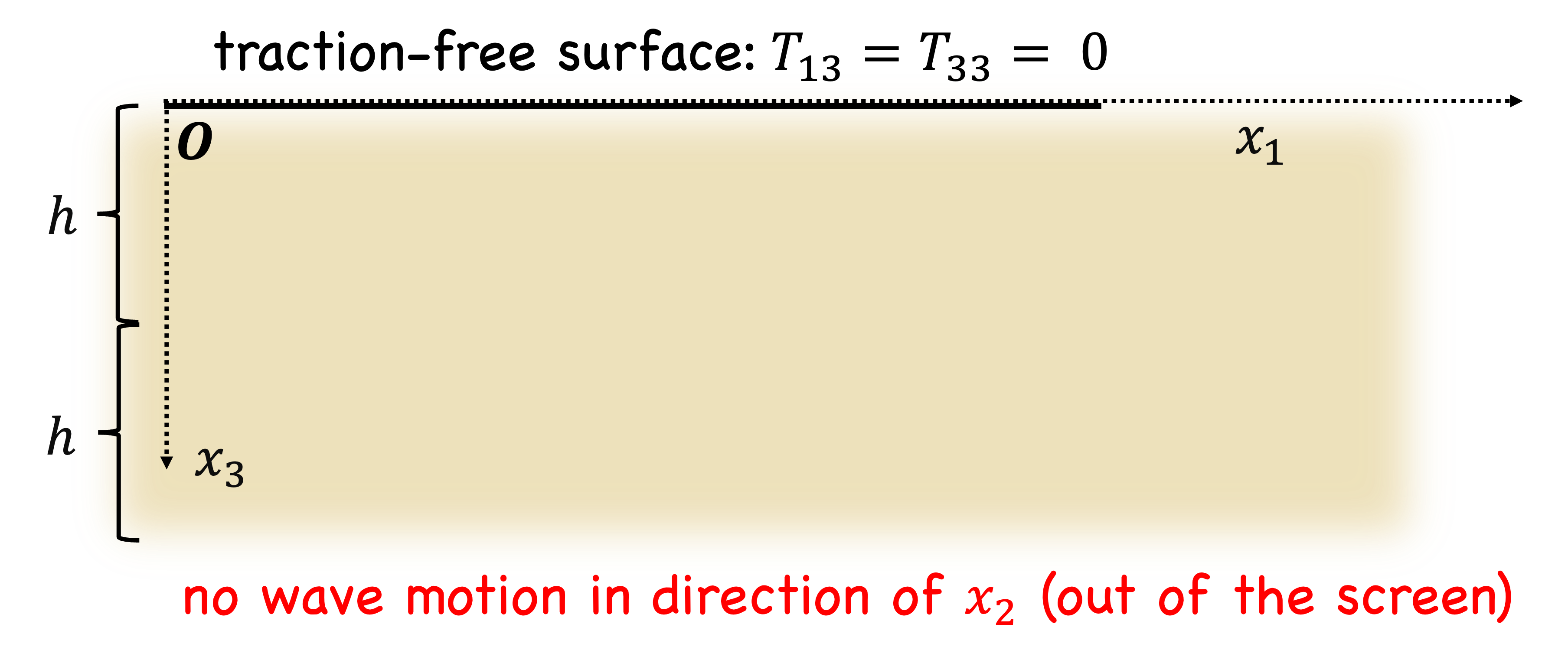
Consider an elastic half-space with a traction-free surface. Limit wave propagation to two dimensions, where \(x_3\) points downward, and \(x_1\) is oriented along the surface of the half-space: This "plane-strain" condition requires that there is no displacement in the \(x_2\) direction, i.e., \(u_2 = 0\). What are the potential functions \(\phi\) and \(\vec{\psi}\) that describe the displacement field \(\vec{u} = \vec{\nabla} \phi + \vec{\nabla}\times \vec{\psi}\)? [answer]

Note that in index notation, \[\vec{\nabla}\phi = \phi_{,1}\hat{x}_1 + \phi_{,2}\hat{x}_2 + \phi_{,3}\hat{x}_3 \] and \[\vec{\nabla}\times\vec{\psi} = (\psi_{3,2} - \psi_{2,3})\hat{x}_1 + (\psi_{1,3}-\psi_{3,1})\hat{x}_2 + (\psi_{2,1}-\psi_{1,2})\hat{x}_3\,.\] The component \(u_2\) of \(\vec{u} = \vec{\nabla} \phi + \vec{\nabla}\times \vec{\psi}\) must vanish. To achieve this, \(\phi\) cannot depend on \(x_2\), and \({\psi}_1 = \psi_3 = \text{ constant } = 0\). Thus \(\vec{\psi} = \psi \hat{x}_2\). This gives the displacement components \begin{align*} u_1 &= \phi_{,1} - \psi_{,3}\\ u_3 &= \phi_{,3} + \psi_{,1}\,. \end{align*}
Seek a solution to the compressional wave equation \(\nabla^2 \phi - \ddot{\phi}/c_L^2 = 0\) and the shear wave equation \(\nabla^2 \psi - \ddot{\psi}/c_T^2 = 0\) by assuming the form \(\phi = A(x_3)e^{j(\omega t - kx_1)}\) and \(\psi = B(x_3)e^{j(\omega t - kx_1)}\). [answer]

Inserting the forms of solution into the corresponding wave equations (see here for details) gives \[A(x_3)'' + k^2[(c_R/c_L)^2 - 1] A(x_3) = 0\] and \[B(x_3)'' + k^2[(c_R/c_T)^2 - 1] B(x_3) = 0\,,\] where \(c_R = \omega/k\) (the Rayleigh wave speed).

The solution to the above ODEs is \begin{align*} A(x_3) &= Ae^{\pm kqx_3},\quad q = \sqrt{1-(c_R/c_L)^2} \\ B(x_3) &= Be^{\pm ksx_3},\quad s = \sqrt{1-(c_R/c_T)^2} \,. \end{align*} Substituting these results into the assumed form of solution gives \begin{align*} \phi(\vec{x},t) &= A e^{-kqx_3}e^{j(\omega t - kx_1)}\\ \psi(\vec{x},t) &= B e^{-ksx_3}e^{j(\omega t - kx_1)}\,. \end{align*}
The boundary conditions of a traction-free surface in 2D are that the normal and shear components of the stress vanish: \begin{align*} T_{13} &= 2\mu E_{13} = 0\\ T_{33} &= (\lambda + 2\mu)E_{33} + \lambda E_{11} = 0\,. \end{align*} Use the definition of the linear strain tensor to write these relations in terms of the displacements. Use the displacement potentials calculated previously to obtain a characteristic equation that satisfies these boundary conditions. Hint: Define \(r \equiv s^2 + 1 = 2- (c_R/c_T)^2\). Answer: \(r^2 - 4sq = 0\). [answer]

Using the linear strain tensor, \(E_{mn} = \frac{1}{2}(u_{m,n} + u_{n,m})\), the boundary conditions are written in terms of the displacements. \begin{align*} T_{13} &= 2\mu E_{13} = 2\mu (u_{1,3} + u_{3,1})/2 = 0\\ T_{33} &= (\lambda + 2\mu)E_{33} + \lambda E_{11} = \lambda u_{1,1} + (\lambda+2\mu) u_{3,3}= 0\,. \end{align*} Using the displacement potentials \begin{align*} \phi(\vec{x},t) &= A e^{-kqx_3}e^{j(\omega t - kx_1)}\\ \psi(\vec{x},t) &= B e^{-ksx_3}e^{j(\omega t - kx_1)}\,. \end{align*} the displacements are found to be \begin{align*} u_1 &= \phi_{,1} - \psi_{,3} \\ &=(-jk A e^{-kqx_3} + ks B e^{-ksx_3}) e^{j(\omega t - kx_1)}\\ u_3 &= \phi_{,3} + \psi_{,1}\\ &= (-kq A e^{-kqx_3} -jk B e^{-ksx_3}) e^{j(\omega t - kx_1)} \end{align*} The derivatives of the displacement are taken in preparation for satisfying the boundary conditions: \begin{align*} u_{1,1} &= (-k^2 A e^{-kqx_3} - jk^2s B e^{-ksx_3}) e^{j(\omega t - kx_1)}\\ u_{1,3} &= (jk^2q A e^{-kqx_3} - k^2s^2 B e^{-ksx_3}) e^{j(\omega t - kx_1)}\\ u_{3,1} &= (jk^2q A e^{-kqx_3} -k^2 B e^{-ksx_3}) e^{j(\omega t - kx_1)}\\ u_{3,3} &= (k^2q^2 A e^{-kqx_3} +jk^2s B e^{-ksx_3}) e^{j(\omega t - kx_1)} \end{align*} Inserting the above derivatives in the continuity conditions at the boundary \(x_3=0\) gives \begin{align*} T_{13} = 2\mu (u_{1,3} + u_{3,1})/2 &= 0\\ \implies jk^2q A - k^2s^2 B + jk^2q A -k^2 B &= 0\\ 2js A - (1+ s^2) B &= 0 \end{align*} Recall that \(s^2 = 1- (c_R/c_T)^2\) and define \(r \equiv s^2 + 1 = 2- (c_R/c_T)^2\), giving \begin{equation}\label{firstRayleighBC}\tag{i} 2jq A - r B = 0\,. \end{equation} Meanwhile, the other boundary condition gives \begin{align*} 0 &= T_{33} = \lambda u_{1,1} + (\lambda+2\mu) u_{3,3}\\ &\implies \lambda(-k^2 A - jk^2s B) + (\lambda+2\mu)(k^2q^2 A +jk^2s B)\\ &= \lambda(- A - js B) + (\lambda+2\mu)(q^2 A +js B)\\ &=- \lambda A - js \lambda B + (\lambda+2\mu)q^2 A +js (\lambda+2\mu) B \\ &=[(\lambda+2\mu)q^2 - \lambda] A + js [-\lambda + (\lambda+2\mu)] B \\ &=[(\lambda+2\mu)q^2 - \lambda] A - 2js\mu B \end{align*} Dividing the last equation above by \(\mu\) gives \begin{align*} [q^2(\lambda+2\mu)/\mu - \lambda/\mu] A - 2js B &=0 \end{align*} Note that \((\lambda+2\mu)/\mu = c_L^2/c_T^2\), and recall that \(q^2 = 1-c_R^2/c_L^2\). Write \[\lambda/\mu = (\lambda+2\mu)/\mu - 2\] in the square brackets, giving \begin{align*} 0 &= [q^2(\lambda+2\mu)/\mu - (\lambda+2\mu)/\mu + 2] A - 2js B \\ &= [(1-c_R^2/c_L^2) (c_L/c_T)^2 - (c_L/c_T)^2 + 2] A - 2js B \\ &=[ (c_L/c_T)^2 - c_R^2/c_T^2 - (c_L/c_T)^2 + 2] A - 2js B \\ &=[2- c_R^2/c_T^2 ] A - 2js B \end{align*} Identifying \(r= 2- (c_R/c_T)^2\) gives \begin{equation}\label{secondRayleighBC}\tag{ii} r A - 2js B =0 \end{equation} (Only someone who truly loves waves would have the patience for this kind of algebra). Combining equations (\ref{firstRayleighBC}) and (\ref{secondRayleighBC}) gives the system of linear equations \begin{align*} \begin{pmatrix} 2jq & -r\\ r & -2js \end{pmatrix} \begin{pmatrix} A\\ B \end{pmatrix} =\begin{pmatrix} 0\\ 0 \end{pmatrix}\,. \end{align*} Nontrivial solutions (\(A \neq 0, B\neq 0\)) exist for the case when the \(2\times 2\) matrix above is not invertible, i.e., \begin{align*} \det \begin{pmatrix} 2jq & -r\\ r & -2js \end{pmatrix} &=0\\ r^2 - 4sq &= 0\,. \end{align*}
Define \(\eta \equiv c_R/c_T\) and \(\zeta = c_T/c_L\). This gives \begin{align*} r &= 2 - (c_R/c_T)^2 = 2-\eta^2,\\ s &= \sqrt{1 - (c_R/c_T)^2} = \sqrt{1-\eta^2}\\ q &= \sqrt{1 - (c_R/c_L)^2} = \sqrt{1-\eta^2 \zeta^2}. \end{align*} Write the characteristic equation for Rayleigh waves at a traction-free surface, \(r^2 - 4sq = 0\), in terms of these parameters. How many roots does this equation have, and how many of them are physical? Answer: \[\eta^6 - 8\eta^4 + 8\eta^2 (3- 2\zeta^2) + 16(\zeta^2 - 1) = 0.\] (I am having a hard time showing this. Let me know if you know how it's done.) [answer]

I can't figure this out :(

The 6th order equation generally has six complex roots, but only the real positive roots are physical.
Are Rayleigh waves dispersive? [answer]

Rayleigh waves are not dispersive since \(\eta\) is only a function of the Poisson's ratio.
In what case can a Rayleigh wave travel along a curved surface? [answer]

A Rayleigh wave travel along a curved surface if the wavelength is much smaller than the radius of curvature.

Waves in plates

This section covers waves in plates of two types: horizontally polarized shear waves and Lamb waves. Note that Lamb waves were not discussed in depth in class, and the relevant homework assignments were numerical exercises. Their derivation is similar to that for Rayleigh waves.

What is an SH wave? How are they different from Lamb waves? [answer]

An SH wave is a "horizontally polarized shear wave," which are waves with a strain orthogonal to the direction of propoagation (studied here in a plate with traction-free surfaces). Often the direction of polarization is chosen to be in the direction of \(\hat{x}_3\). SH waves have the same form as acoustic waves. Lamb waves are waves in plates with traction-free surfaces, but with plane strain conditions (I am not sure if this true about all Lamb waves, but it is true for the Lamb waves in Dr. Haberman's notes). That is, Lamb waves neglect SH waves.
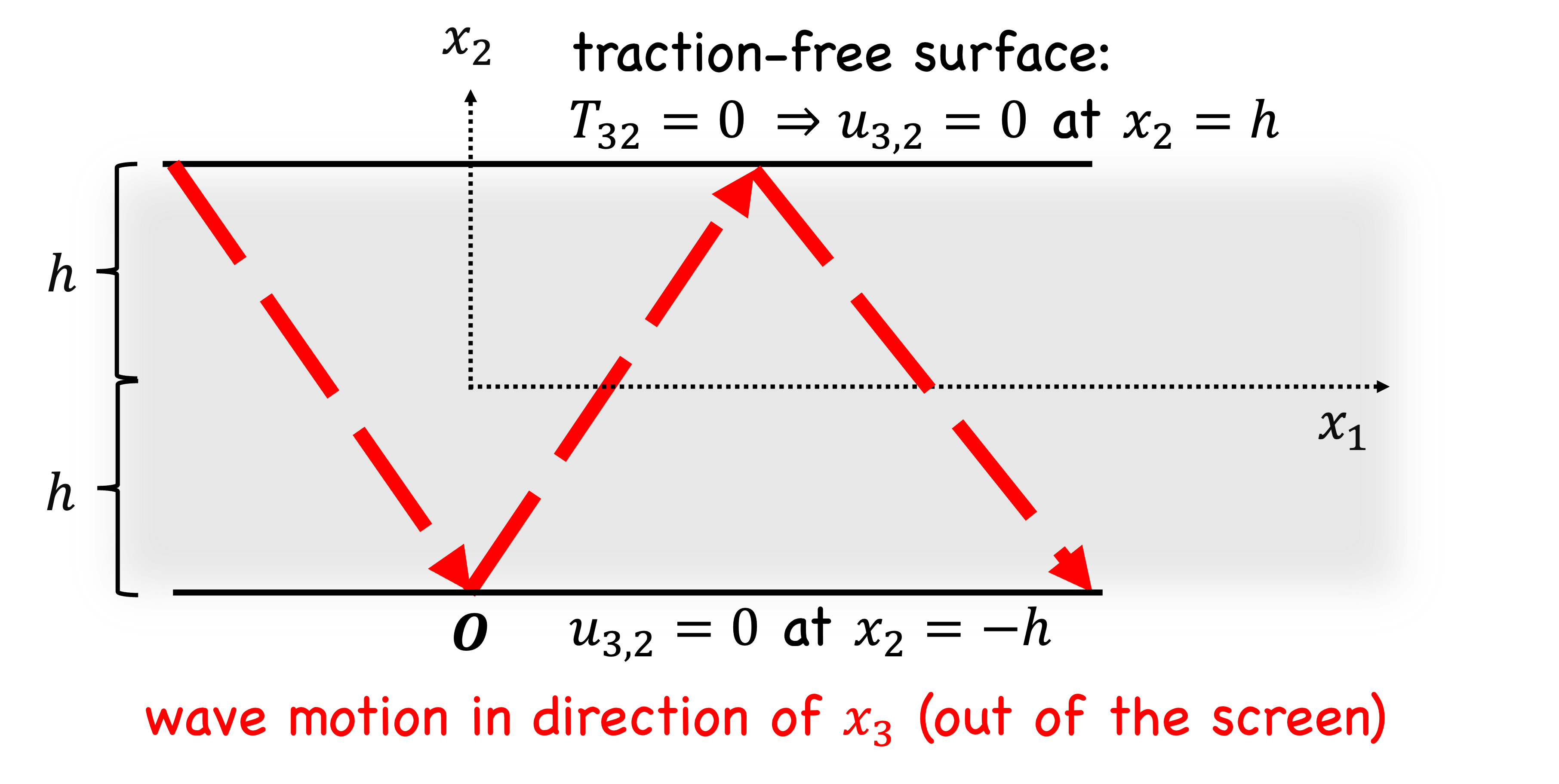
The wave equation for SH waves is very similar to the acoustic wave equation in 2D: \[\frac{\partial^2 u_3}{\partial x_1^2} + \frac{\partial^2 u_3}{\partial x_2^2} -\frac{1}{c_T^2}\frac{\partial^2 u_3}{\partial t^2} = 0\,.\] Assume the wave motion is of the form \(u_3(x_1,x_2,t) = f(x_2) e^{j(\omega t - kx_1)}\), where the coordinates are defined below. Obtain the function \(f(x_2)\), where \(q = \sqrt{k_T^2 - k^2}\). What kinds of modes does the application of the boundary conditions at \(h\) and \(-h\) give rise to? [answer]

The function \(f(x_2)\) must be harmonic, as can be seen by inspection from the wave equation (or, formally, by separation of variables): \[f(x_2) = B_1 \sin (qx_2) + B_2\cos(qx_2)\,.\] \(q\) is determined by application of the boundary conditions of the traction-free surface, which require that the derivative of \(f\) vanishes at \(x = h\) and \(x = -h\): \begin{align*} B_1\cos(qh) + B_2\sin(qh) &= 0\\ B_1\cos(-qh) + B_2\sin(-qh) &= 0\,, \end{align*} or, using the even and odd properties of the trigonometric functions, \begin{align*} B_1\cos(qh) + B_2\sin(qh) &= 0\\ B_1\cos(qh) - B_2\sin(qh) &= 0\,. \end{align*} Both equations are satisfied by \begin{align} B_1 &= 0,\quad qh = \frac{n\pi}{2},\quad n = 0,2,4\dots \tag*{even}\\ B_2 &= 0,\quad qh = \frac{n\pi}{2},\quad n = 1,3,5\dots\,.\tag*{odd} \end{align}

Evidently, the application of the boundary conditions gives rise to "symmetric" and "antisymmetric" modes, named for the symmetry/antisymmetry of the even/odd \(n\) modes about the midplane.
Given that \(q_n = n\pi/2h\), obtain the dispersion relation \(\Omega(K)\), where \(\Omega = 2h\omega/\pi c_T\) is the dimensionless frequency, and \(K = 2kh/\pi\) is the dimensionless wavenumber. Qualitatively describe the dispersion relation. Obtain the dimensionless group and phase speeds of the SH waves. [answer]

Solve \[q_n^2= (n\pi/2h)^2 = k_T^2 - k^2\] for \(k^2 = \omega/c_T\) and divide by \((\pi/2h)^2\) to obtain \[n^2 + (2kh/\pi)^2 = (2h\omega/\pi c_T)^2,\] which gives \[n^2 + K^2 = \Omega^2\,.\]

The dispersion relation consists of an infinite number of continuous branches, each corresponding to an integer value of \(n\). The lowest (\(n=0\)) mode is non-dispersive, and all the heigher order modes are hyperbolas with \(\Omega = K\) asymptotes.

The dimensionless phase speed is \[\frac{\Omega}{K} = \pm \sqrt{(n/K)^2 + 1},\] and the dimensionless group speed is \[\frac{d\Omega}{dK} = \pm \frac{1}{\sqrt{1 + (n/K)^2}}\,.\]
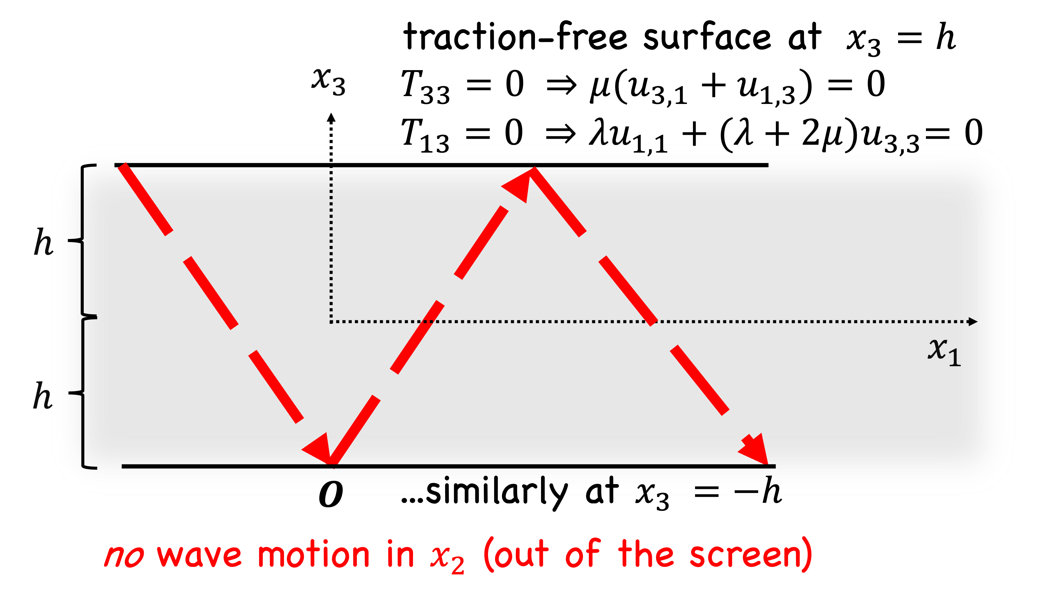
Outline the derivation for Lamb waves between two layers, where the coordinates are as defined below. Limit the derivation to plane strain, i.e., \(u_2 = 0\), and do not attempt to satisfy the boundary conditions. [answer]

First note that for plane-strain propagation (see question 1 of the Rayleigh wave section) \begin{align*} u_1 &= \phi_{,1} - \psi_{,3}\\ u_3 &= \phi_{,3} - \psi_{,1}\,. \end{align*} Similar to the Rayleigh wave problem, it is assumed that the potentials have the form \begin{align*} \phi(\vec{x},t) &= f(x_3) e^{j(\omega t - kx_1)}\\ \psi(\vec{x},t) &= g(x_3) e^{j(\omega t - kx_1)}\,. \end{align*} To determine \(f(x_3)\) and \(g(x_3)\), the potentials are inserted into their respective wave equations, \begin{align*} \phi_{,11}+ \phi_{,33} - \frac{1}{c_L^2}\ddot{\phi} &= 0\\ f''(x_3) + (\omega^2/c_L^2 - k^2)f(x_3) &= 0 \end{align*} and \begin{align*} \psi_{,11}+ \psi_{,33} - \frac{1}{c_T^2}\ddot{\psi} &= 0\\ g''(x_3) + (\omega^2/c_T^2 - k^2)g(x_3) &= 0\,. \end{align*} Solving the above second-order ODEs gives \begin{align*} f(x_3) &= A_1 \sin (px_3) + A_2 \cos (px_3)\,,\quad p = k\sqrt{(k_L/k)^2 -1} \,,\\ g(x_3) &= B_1 \sin (qx_3) + B_2 \cos (qx_3)\,, \quad q = k\sqrt{(k_T/k)^2 -1} \,. \end{align*} The displacements are calculated by \(u_1 = \phi_{,1} - \psi_{,3}\) and \(u_3 = \phi_{,3} - \psi_{,1}\). As is the case with the SH waves, \(u_1\) and \(u_3\) can be classified as symmetric and antisymmetric (about the midplane of the plate).

The boundary conditions are that the normal and shear stresses vanish at both \(x_3=h\) and \(x_3 = -h\): \begin{align*} T_{33} &= 0\, \implies \lambda u_{1,1} + (\lambda + 2\mu ) u_{3,3} = 0\\ T_{13} &= 0\, \implies \mu (u_{1,3} + u_{3,1})\,. \end{align*} Application of the boundary conditions to the even and odd modes results in the so-called Rayleigh-Lamb relations. These relations must be solved numerically for almost all practical cases.